Bag of Words and N-grams

Bag of Words (BOW)#

Let us consider a corpus as follows:

corpus = [
    "I saw a blue bird",
    "The blue bird was sitting on a tree",
    "The blue bird flew away",
]

Here, we have three documents:
D1 -> I saw a blue bird
D2 -> The blue bird was sitting on a tree
D3 -> The blue bird flew away

Preprocessing: Removing stopwords#

After removing the stopwords, our documents will be:
D1 -> saw blue bird
D2 -> blue bird sitting tree
D3 -> blue bird flew away

Note

To keep things simple, we did not apply other pre-processing techniques such as lowering, stemming or lemmatization. Only stopwords was applied to lower vocabulary size for easier explaination and understanding.

Step 1: Determine vocabulary#

Our vocabulary from these three documents will be:

['saw', 'blue', 'bird', 'sitting', 'tree', 'flew', 'away']

Step 2: Calculating Frequency#

To vectorize our documents, all we have to do is count how many times each word (we call them features) appears

We, thus, have our vectors of length 7 for each document as follows:

D1 -> [1, 1, 1, 0, 0, 0, 0]
D2 -> [0, 1, 1, 1, 1, 0, 0]
D3 -> [0, 1, 1, 0, 0, 1, 1]

Binary Bag of Words (BOW)#

Suppose we have a slightly modified corpus and our D1 as one more word ‘blue’ in it:

D1 -> saw blue bird blue
D2 -> blue bird sitting tree
D3 -> blue bird flew away

Applying BOW to the above will give us the following vectors:

D1 -> [1, 2, 1, 0, 0, 0, 0]
D2 -> [0, 1, 1, 1, 1, 0, 0]
D3 -> [0, 1, 1, 0, 0, 1, 1]

For Binary BOW, even if a word occurs more than once in our vocabulary, the count remain as 1:

D1 -> [1, 1, 1, 0, 0, 0, 0]
D2 -> [0, 1, 1, 1, 1, 0, 0]
D3 -> [0, 1, 1, 0, 0, 1, 1]

Advantages#

• Simple and intuitive - The strength of BOW lies in it’s simplicity, which can be used in tasks like Text Classification

Disadvantages#

• Creates sparse matrices - although better than OHE, the computational complexity doesn’t improve that much
• Out of Vocabulary issue persists
• Semantic meaning is still not captured

Example Code#

from sklearn.feature_extraction.text import CountVectorizer

# Define the corpus
corpus = [
    "saw blue bird",
    "blue bird sitting tree",
    "blue bird flew away",
]

# Create an instance of CountVectorizer
vectorizer = CountVectorizer(binary=True) # This parameter generates Binary BOW, default is False

# Fit and transform the corpus to obtain the bag-of-words representation
bow_matrix = vectorizer.fit_transform(corpus)

# Get the feature names (words) from the vectorizer
feature_names = vectorizer.get_feature_names_out()

# Convert the bag-of-words matrix to a dense array for easier visualization
dense_bow_matrix = bow_matrix.toarray()

# Display the bag-of-words matrix
print("Bag-of-Words Matrix:")
print(dense_bow_matrix)

# Display the feature names
print("\nFeature Names:")
print(feature_names)

Output

 Bag-of-Words Matrix:
 [[0 1 1 0 1 0 0]
  [0 1 1 0 0 1 1]
  [1 1 1 1 0 0 0]]

 Feature Names:
 ['away' 'bird' 'blue' 'flew' 'saw' 'sitting' 'tree']

Note

The features might seem to be appearing at random. This is because, CountVectorizer arranges the features in alphabetical order.

One can also set the maximum number of features to be considered. Setting the parameter ‘max_features’ ensures consideration of top ‘max_features’ ordered by term frequency (more on that in the next chapter) across the corpus. Otherwise, all features are used.

vectorizer = CountVectorizer(max_features=3)

Output

 Bag-of-Words Matrix:
 [[0 1 1]
  [0 1 1]
  [1 1 1]]

 Feature Names:
 ['away' 'bird' 'blue']

It might also be helpful to figure out the index of the features, which can be done as follows:

vectorizer.vocabulary_

Output

 {'saw': 4, 'blue': 2, 'bird': 1, 'sitting': 5, 'tree': 6, 'flew': 3, 'away': 0}

N-grams#

With n-grams, we start considering combination of features. They are basically a set of co-occurring words within a given window and when computing the n-grams you typically move one word forward (although you can move X words forward in more advanced scenarios).

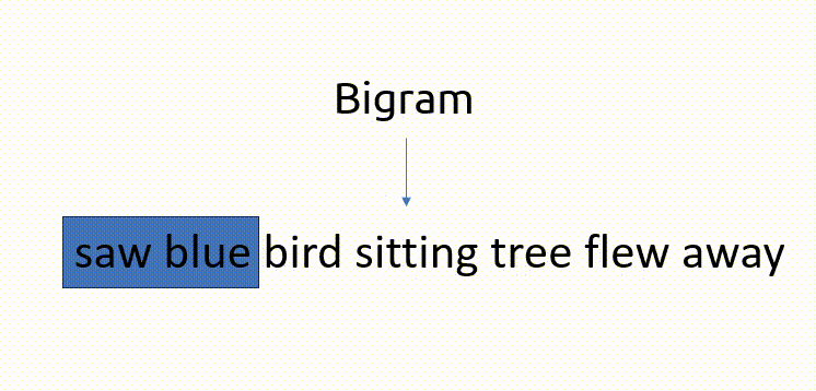
Below is an example of bigram:

Similarly, for trigram, we consider three co-occuring words and so on.

N-gram is used to consider words in their real order so we can get an idea about the context of the particular word

Step 1: Determine Vocabulary#

From our example corpus above, applying bigram and re-creating the vocabulary would give us

['saw', 'blue', 'bird', 'sitting', 'tree', 'flew', 'away', 'saw blue', 'blue bird', 'bird sitting', 'sitting tree', 'tree flew', 'flew away']

Step 2: Calculating Frequency#

Similar to how we calculated the frequency before

Note

The other bigrams are not here due to lack of space :(

And our vectors for each document will be:

D1 -> [1, 1, 1, 0, 0, 0, 0, 1, 1, 0, 0, 0, 0]
D2 -> [0, 1, 1, 1, 1, 0, 0, 0, 1, 1, 1, 0, 0]
D3 -> [0, 1, 1, 0, 0, 1, 1, 0, 1, 0, 0, 0, 1]

Advantages#

• Semantic meaning is somewhat captured

Disadvantages#

• Increases the sparsity of the matrix

Example Code#

We can apply n-grams to our above code by adding a parameter ’ngram_range=(1,3)’ to the CountVectorizer:

vectorizer = CountVectorizer(ngram_range=(1,3))

Output

 Bag-of-Words Matrix:
 [[0 1 0 0 0 0 1 1 0 0 0 0 1 1 1 0 0 0]
  [0 1 0 0 1 1 1 1 0 1 0 0 0 0 0 1 1 1]
  [1 1 1 1 0 0 1 1 1 0 1 1 0 0 0 0 0 0]]

 Feature Names:
 ['away' 'bird' 'bird flew' 'bird flew away' 'bird sitting'
  'bird sitting tree' 'blue' 'blue bird' 'blue bird flew'
  'blue bird sitting' 'flew' 'flew away' 'saw' 'saw blue' 'saw blue bird'
  'sitting' 'sitting tree' 'tree']

Note

Notice how features are selected from single words, bigrams and trigrams. Defining ngram_range as ’ngram_range=(2,2)’ will only consider bigrams and ’ngram_range=(3,3)’ will only consider trigrams and so on